A simple modeling workflow
Overview
Teaching: 20 min
Exercises: 20 minObjectives
re-format data for model input
view the model
predict function
model evaluation
thresholds
 .
.
5.0 Prepare occ & raster
library("raster")
library("dismo")

if(!file.exists("data/occ_raw.rdata")){
  occ_raw <- gbif(genus="Dasypus",species="novemcinctus",download=TRUE)
  save(occ_raw,file = "data/occ_raw.rdata")
}else{
  load("data/occ_raw.rdata")
}
occ_clean <- subset(occ_raw,(!is.na(lat))&(!is.na(lon)))
occ_unique <- occ_clean[!duplicated( occ_clean[c("lat","lon")]  ),]
occ_unique_specimen <- subset(occ_unique, basisOfRecord=="PRESERVED_SPECIMEN")
occ_final <- subset(occ_unique_specimen, year>=1950 & year <=2000)
coordinates(occ_final) <- ~ lon + lat
myCRS1 <- CRS("+init=epsg:4326") # WGS 84
crs(occ_final) <- myCRS1

if( !file.exists( paste0("data/bioclim/bio_10m_bil.zip")   )){
  utils::download.file(url="http://biogeo.ucdavis.edu/data/climate/worldclim/1_4/grid/cur/bio_10m_bil.zip",
                       destfile="data/bioclim/bio_10m_bil.zip"   )
  utils::unzip("data/bioclim/bio_10m_bil.zip",exdir="data/bioclim")
}

clim_list <- list.files("data/bioclim/",pattern=".bil$",full.names = T)
clim <- raster::stack(clim_list)

occ_buffer <- buffer(occ_final,width=4*10^5) #unit is meter
clim_mask <- mask(clim, occ_buffer)
5.1 Re-format data input for Maxent
The data input can either be spatial (i.e. spatial points + rasters) or *tabular (data frame).
Here is an example of using spatial data:
cat(class(clim_mask)," ", class(occ_final))
RasterBrick SpatialPointsDataFrame
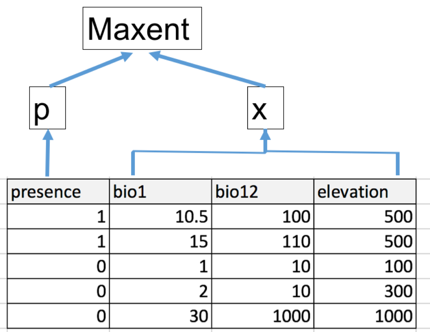
m0 <- maxent(x=clim_mask,p=occ_final)
Warning in .local(x, p, ...): 2 (0.39%) of the presence points have NA
predictor values
However, using spatial data input will make the model less under control. So if you want more control of the modeling process, it is recommended to prepare data in a tabular format. The ideal format is as following:
 .
.
Here, we extract environmental conditions for occurrences (training, and testing) and background points, and merge them by row.
set.seed(1)
bg <- sampleRandom(x=clim_mask,
                   size=10000,
                   na.rm=T, #removes the 'Not Applicable' points
                   sp=T) # return spatial points

set.seed(1)

# randomly select 50% for training
selected <- sample(  1:nrow(occ_final),  nrow(occ_final)*0.5)

occ_train <- occ_final[selected,] # this is the selection to be used for model training
occ_test <- occ_final[-selected,] # this is the opposite of the selection which will be used for model testing


# extracting env conditions for training occ from the raster stack;
# a data frame is returned (i.e multiple columns)
env_occ_train <- extract(clim,occ_train)

# env conditions for testing occ
env_occ_test <- extract(clim,occ_test)

# extracting env conditions for background
env_bg <- extract(clim,bg)

#combine the conditions by row
myPredictors <- rbind(env_occ_train,env_bg)

# change matrix to dataframe
myPredictors <- as.data.frame(myPredictors)
head(myPredictors)
  bio1 bio10 bio11 bio12 bio13 bio14 bio15 bio16 bio17 bio18 bio19 bio2
1  236   275   193  1309   158    44    35   453   160   418   160  118
2  197   220   166  1358   256    23    70   683    86   625   107  112
3  180   270    86  1232   129    68    15   350   244   263   324  127
4  250   285   209   751   178     1   106   517     8   393    69  105
5  121   248    -8   593    90    11    56   262    42   249    42  148
6  240   243   236  4149   633    97    50  1690   372   665  1690  106
  bio3 bio4 bio5 bio6 bio7 bio8 bio9
1   57 3279  336  131  205  270  193
2   63 2205  274   98  176  220  166
3   39 7168  340   15  325  220  265
4   57 3052  330  147  183  283  240
5   34 9906  339  -93  432  222   -8
6   87  304  301  180  121  236  238
Maxent reads a 1 as presence and 0 as background. Thus, we need to assign a 1 to the training environmental conditions and a 0 for the background.We create a set of rows with the same number as the training and testing data, and put the value of “1” for each cell and a “0” for background. We combine the “1”s and “0”s into a vector.
# repeat the number 1 as many times as the number of rows in p,
# and repeat 0 for the rows of background points
myResponse <- c(rep(1,nrow(env_occ_train)),
                rep(0,nrow(env_bg)))

# (rep(1,nrow(p)) creating the number of rows as the p data set to
# have the number '1' as the indicator for presence; rep(0,nrow(a))
# creating the number of rows as the a data set to have the number
# '0' as the indicator for absence; the c combines these ones and
# zeros into a new vector that can be added to the Maxent table data
# frame with the environmental attributes of the presence and absence locations

mod <- maxent(x=myPredictors,p=myResponse)
5.2 View the model
mod@lambdas
  [1] "bio1, 0.0, -17.0, 288.0"
  [2] "bio10, 0.0, 28.0, 323.0"
  [3] "bio11, 0.0, -115.0, 279.0"
  [4] "bio12, 0.0, 0.0, 7507.0"
  [5] "bio13, 0.0, 0.0, 789.0"
  [6] "bio14, 0.0, 0.0, 471.0"
  [7] "bio15, 0.26763106606745934, 0.0, 179.0"
  [8] "bio16, 0.0, 0.0, 2220.0"
  [9] "bio17, 0.0, 0.0, 1446.0"
 [10] "bio18, 0.0, 0.0, 1862.0"
 [11] "bio19, 0.0, 0.0, 1833.0"
 [12] "bio2, 0.0, 49.0, 197.0"
 [13] "bio3, 0.0, 24.0, 92.0"
 [14] "bio4, 0.0, 153.0, 11700.0"
 [15] "bio5, 0.0, 91.0, 420.0"
 [16] "bio6, 0.0, -218.0, 238.0"
 [17] "bio7, 0.0, 67.0, 458.0"
 [18] "bio8, 0.0, -109.0, 318.0"
 [19] "bio9, 0.0, -93.0, 290.0"
 [20] "bio11^2, -0.9050993113644507, 0.0, 77841.0"
 [21] "bio6^2, -0.23747649426508424, 0.0, 56644.0"
 [22] "bio9^2, 0.4275995833412999, 0.0, 84100.0"
 [23] "bio1*bio4, 0.4275531776699976, -133807.0, 1744554.0"
 [24] "bio10*bio4, 1.2031027271578127, 25020.0, 2573018.0"
 [25] "bio11*bio6, -0.30462690571479045, -3264.0, 63800.0"
 [26] "bio11*bio8, -0.3250871769514228, -19623.0, 80352.0"
 [27] "bio12*bio15, 0.19172246501526033, 0.0, 293293.0"
 [28] "bio13*bio15, 1.9606573117627615, 0.0, 65130.0"
 [29] "bio14*bio15, 1.580649741721404, 0.0, 8100.0"
 [30] "bio18*bio2, -1.2542634205271663, 0.0, 180614.0"
 [31] "bio18*bio7, -0.33814584317352503, 0.0, 247450.0"
 [32] "bio19*bio4, -1.6067710599902456, 0.0, 5057568.0"
 [33] "bio3*bio4, -0.1353239541968972, 13464.0, 376200.0"
 [34] "bio3*bio5, -0.18718091328019476, 5100.0, 30096.0"
 [35] "bio4*bio8, 1.0999308089617332, -857939.0, 2533188.0"
 [36] "(116.5<bio1), 1.7050295973145897, 0.0, 1.0"
 [37] "(264.5<bio10), 0.35291115992405353, 0.0, 1.0"
 [38] "(391.5<bio12), 0.5268415414479714, 0.0, 1.0"
 [39] "(464.5<bio12), 0.2809049348106028, 0.0, 1.0"
 [40] "(702.5<bio4), 0.02142587052662699, 0.0, 1.0"
 [41] "(181.5<bio6), -0.0035686507209030487, 0.0, 1.0"
 [42] "(94.5<bio15), 0.38328645908332803, 0.0, 1.0"
 [43] "(113.5<bio7), 0.27630610703640396, 0.0, 1.0"
 [44] "(44.5<bio3), -0.24341708475932264, 0.0, 1.0"
 [45] "(169.5<bio2), -0.8805244643493182, 0.0, 1.0"
 [46] "(180.5<bio6), -0.18330370526478784, 0.0, 1.0"
 [47] "(108.5<bio7), 0.5002170217141941, 0.0, 1.0"
 [48] "(89.5<bio15), 0.26746743942617796, 0.0, 1.0"
 [49] "(161.5<bio2), -0.5999534648855973, 0.0, 1.0"
 [50] "(168.5<bio1), 3.879523444910368E-4, 0.0, 1.0"
 [51] "(644.5<bio18), 0.4529722070472205, 0.0, 1.0"
 [52] "(6.5<bio17), 0.3377788196645386, 0.0, 1.0"
 [53] "(83.5<bio2), 0.7336888159816374, 0.0, 1.0"
 [54] "(200.5<bio10), -0.1446986549956838, 0.0, 1.0"
 [55] "(2375.0<bio12), 0.21713583667210642, 0.0, 1.0"
 [56] "(9534.0<bio4), 0.30445606508477613, 0.0, 1.0"
 [57] "(922.5<bio18), -0.8194849771088258, 0.0, 1.0"
 [58] "(166.5<bio14), -0.35761122017187547, 0.0, 1.0"
 [59] "(90.5<bio14), 0.012535558287089285, 0.0, 1.0"
 [60] "(229.5<bio9), 0.09777880311125317, 0.0, 1.0"
 [61] "(120.5<bio2), -0.11265232152875598, 0.0, 1.0"
 [62] "(147.5<bio2), 0.06641891160954848, 0.0, 1.0"
 [63] "'bio3, -0.6590942767069409, 84.5, 92.0"
 [64] "(118.5<bio2), -0.019175055467032555, 0.0, 1.0"
 [65] "(9.5<bio19), 0.1082764651308983, 0.0, 1.0"
 [66] "`bio1, -2.62299662570326, -17.0, 174.5"
 [67] "(77.5<bio11), 0.1224812869941741, 0.0, 1.0"
 [68] "'bio7, 1.0737412378814233, 388.5, 458.0"
 [69] "`bio17, -0.27527123085013905, 0.0, 42.5"
 [70] "(280.5<bio8), -0.11244424237993984, 0.0, 1.0"
 [71] "(-8.5<bio11), 0.001422384121425667, 0.0, 1.0"
 [72] "`bio12, -2.229804910918043, 0.0, 550.0"
 [73] "'bio11, 1.2088338560623306, 266.5, 279.0"
 [74] "(91.5<bio14), 0.08522175616366341, 0.0, 1.0"
 [75] "`bio15, 0.8558439229257911, 0.0, 18.5"
 [76] "(77.5<bio3), -0.09865537583557168, 0.0, 1.0"
 [77] "(1293.0<bio19), -0.1549899172584807, 0.0, 1.0"
 [78] "(1046.0<bio18), -0.08883760942640118, 0.0, 1.0"
 [79] "'bio6, -0.6530681835192078, 206.5, 238.0"
 [80] "`bio18, -0.2316277231865191, 0.0, 68.5"
 [81] "(269.5<bio8), 0.08085238645569892, 0.0, 1.0"
 [82] "`bio12, -0.3914383332253453, 0.0, 551.5"
 [83] "(358.5<bio5), -0.06183686404200746, 0.0, 1.0"
 [84] "`bio1, -0.39386424700682987, -17.0, 175.5"
 [85] "'bio15, 0.37506121489990235, 78.5, 179.0"
 [86] "`bio15, 0.9011870410944306, 0.0, 19.5"
 [87] "'bio15, 1.366947964804506, 77.5, 179.0"
 [88] "(3279.5<bio4), -0.19794148295258748, 0.0, 1.0"
 [89] "`bio10, 1.7863768328333707, 28.0, 224.5"
 [90] "(283.5<bio8), -0.05669483888677688, 0.0, 1.0"
 [91] "`bio1, -0.27054487968330077, -17.0, 179.5"
 [92] "`bio1, -0.6186742117687162, -17.0, 180.5"
 [93] "(355.5<bio5), -0.08548324725550764, 0.0, 1.0"
 [94] "`bio17, -0.2424451986068934, 0.0, 11.5"
 [95] "(2352.0<bio12), 0.018080484180326595, 0.0, 1.0"
 [96] "(359.5<bio5), -0.029811208725023956, 0.0, 1.0"
 [97] "`bio14, 0.17659628831660346, 0.0, 0.5"
 [98] "`bio17, -0.29706599399834954, 0.0, 10.5"
 [99] "`bio1, -0.9043074623818957, -17.0, 181.5"
[100] "`bio3, 0.1325513115525726, 24.0, 48.5"
[101] "(266.5<bio17), 0.031937862680527056, 0.0, 1.0"
[102] "linearPredictorNormalizer, 6.840459818603078"
[103] "densityNormalizer, 195.11664123760133"
[104] "numBackgroundPoints, 1418"
[105] "entropy, 6.784636178667567"
5.3 Predict function
Running Maxent in R will not automatically make a projection to the data layers, unless you specify this using the parameter projectionlayers. However, we could make projections (to dataframes or raster layers) post hoc using the predict() function.
project model on raster layers (training layers)
# example 1, project to study area [raster]
ped1 <- predict(mod,clim_mask) # studyArea is the clipped rasters
plot(ped1) # plot the continuous prediction

project model on raster layers (whole world maps)
# example 2, project to the world
ped2 <- predict(mod,clim)
plot(ped2)

example 3, project to a dataframe (training occurrences). This returns the predicion value assocaited with a set of condions. In this example, we use the training condition to extract a prediction for each point.
ped3 <- predict(mod,env_occ_train)
head(ped3)
[1] 0.3992549 0.3542653 0.7025179 0.6716762 0.6041868 0.4814589
5.4 Model evaluation
To evaluate models, we use the evaluate() function from the dismo package. Evaluation indices include AUC, TSS, Sensitivity, Specificity, etc.
Model evaluation, where p & a are dataframes (environmental conditions for presences and background points)
Evaluate model with training data
mod_eval_train <- dismo::evaluate(p=env_occ_train,
                                  a=env_bg,
                                  model=mod)
print(mod_eval_train)
class          : ModelEvaluation
n presences    : 303
n absences     : 1122
AUC            : 0.8896257
cor            : 0.5906694
max TPR+TNR at : 0.3927896
Evaluate model with testing data
mod_eval_test <- dismo::evaluate(p=env_occ_test,
                                 a=env_bg,
                                 model=mod)
print(mod_eval_test)
class          : ModelEvaluation
n presences    : 304
n absences     : 1122
AUC            : 0.8279007
cor            : 0.5036505
max TPR+TNR at : 0.393721
compare training & testing AUC
cat( "the training AUC is: ",mod_eval_train@auc ,"\n" )
the training AUC is: 0.8896257
cat( "the testing AUC is: ", mod_eval_test@auc ,"\n" )
the testing AUC is: 0.8279007
5.5 Thresholds
To threshold our continuous predictions of suitability into binary predictions we use the threshold function of the “dismo” package. To plot the binary prediction, we plot the predictions that are larger than the threshold.
Here we use threshold() function to obtain particular thresholds based on evaluation results from the previous step.
thd1 <- threshold(mod_eval_train,stat="no_omission") # 0% omission rate
thd2 <- threshold(mod_eval_train,stat="spec_sens") # highest TSS
thd3 <- threshold(mod_eval_train,stat="sensitivity",sensitivity=0.9) # 10% omission rate, i.e. sensitivity=0.9
thd4 <- threshold(mod_eval_train,stat="sensitivity",sensitivity=0.95) # 5% omission rate, i.e. sensitivity=0.95

# plotting points that are higher than the previously calculated thresholded value
plot(ped1>=thd1)

Challenge: train a Maxent model with dataframe as input, calculate the AUC
–load occurrences & raster layers
–build axxx meterbuffer around occurrences
–maskraster by the buffer of occurrences
–generate random samples from the masked raster usingsampleRandom()
–extract()environmental conditions from raster by points
–re-format the environmental conditions as input for maxent
–train amaxentmodel
–evaluate()the model with testing environmental conditionsSolution
library("raster")
library("dismo")

# prepare spatial occ data
if(!file.exists("data/occ_raw.rdata")){
  occ_raw <- gbif(genus="Dasypus",species="novemcinctus",download=TRUE)
  save(occ_raw,file = "data/occ_raw.rdata")
}else{
  load("data/occ_raw.rdata")
}
occ_clean <- subset(occ_raw,(!is.na(lat))&(!is.na(lon)))
occ_unique <- occ_clean[!duplicated( occ_clean[c("lat","lon")]  ),]
occ_unique_specimen <- subset(occ_unique, basisOfRecord=="PRESERVED_SPECIMEN")
occ_final <- subset(occ_unique_specimen, year>=1950 & year <=2000)
coordinates(occ_final) <- ~ lon + lat
myCRS1 <- CRS("+init=epsg:4326") # WGS 84
crs(occ_final) <- myCRS1

# prepare raster data
if( !file.exists( paste0("data/bioclim/bio_10m_bil.zip")   )){
  utils::download.file(url="http://biogeo.ucdavis.edu/data/climate/worldclim/1_4/grid/cur/bio_10m_bil.zip",
                       destfile="data/bioclim/bio_10m_bil.zip"   )
  utils::unzip("data/bioclim/bio_10m_bil.zip",exdir="data/bioclim")
}

# load rasters
clim_list <- list.files("data/bioclim/",pattern=".bil$",full.names = T)
clim <- raster::stack(clim_list)

occ_buffer <- buffer(occ_final,width=4*10^5) #unit is meter
clim_mask <- mask(clim, occ_buffer)

# extract environmental conditions
set.seed(1)
bg <- sampleRandom(x=clim_mask,
                   size=10000,
                   na.rm=T, #removes the 'Not Applicable' points
                   sp=T) # return spatial points

set.seed(1)

# randomly select 50% for training
selected <- sample(  1:nrow(occ_final),  nrow(occ_final)*0.5)

occ_train <- occ_final[selected,] # this is the selection to be used for model training
occ_test <- occ_final[-selected,] # this is the opposite of the selection which will be used for model testing

# extracting env conditions
env_occ_train <- extract(clim,occ_train)
env_occ_test <- extract(clim,occ_test)

# extracting env conditions for background
env_bg <- extract(clim,bg)

#combine the conditions by row
myPredictors <- rbind(env_occ_train,env_bg)

# change matrix to dataframe
myPredictors <- as.data.frame(myPredictors)

# repeat the number 1 as many times as the number of rows in p, and repeat 0 for the rows of background points
myResponse <- c(rep(1,nrow(env_occ_train)),
                rep(0,nrow(env_bg)))

# training a maxent model with dataframes
mod <- dismo::maxent(x=myPredictors, ## env conditions
                     p=myResponse)   ## 1:presence or 0:absence

# evaluate model based on testing data
mod_eval_test <- dismo::evaluate(p=env_occ_test,
                                 a=env_bg,
                                 model=mod)
mod_eval_test@auc