Occurrence data
Overview
Teaching: 10 min
Exercises: 10 minObjectives
download occurrence data through API.
filter occurrance data.
## "","x"
## "1","data/occ_raw.csv"
2.1 API
~1 billion biodiversity records on GBIF.org
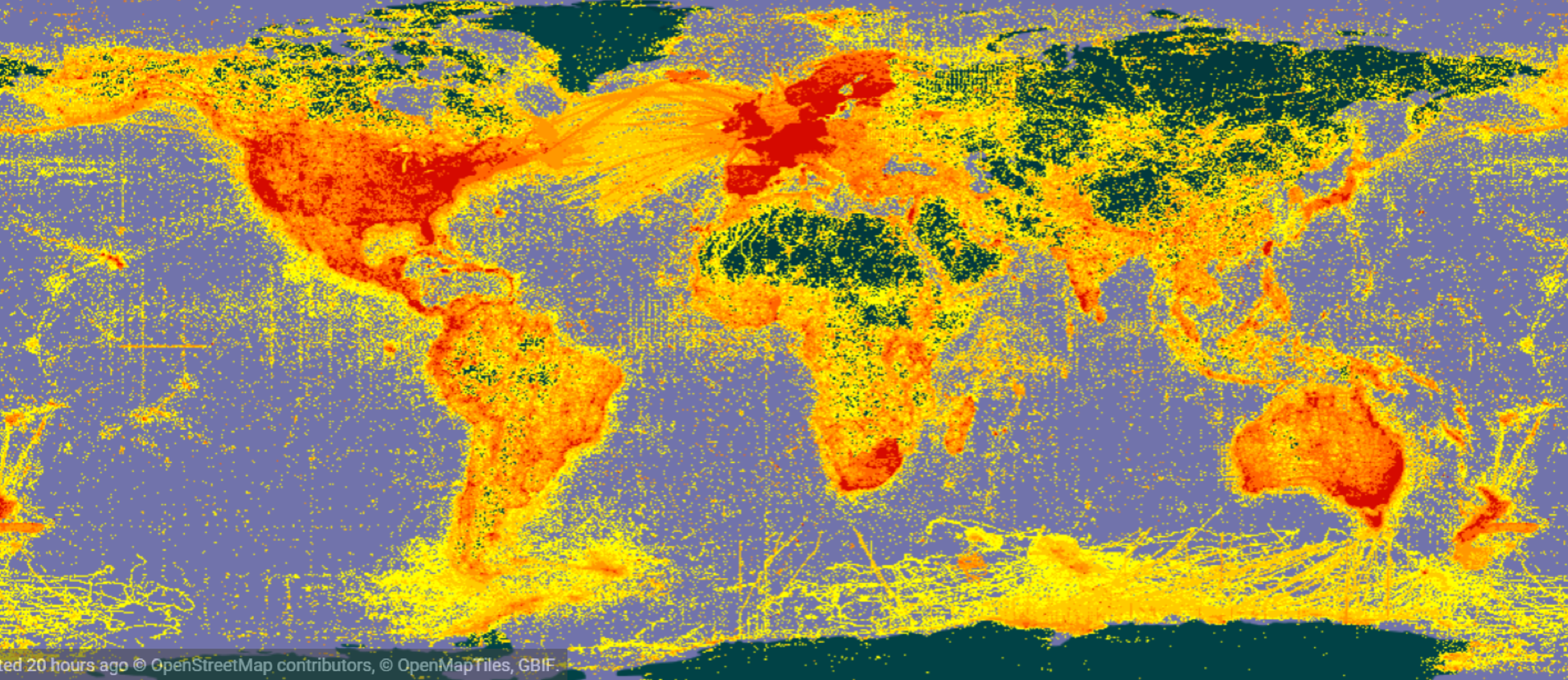 .
.
What is an API looks like?
put this in Chrome/IE: http://api.gbif.org/v1/occurrence/search?year=1800,1899
What is an API? (Application Programming Interface)
API is the acronym for Application Programming Interface, which is a software intermediary that allows two applications to talk to each other. Each time you use an app like Facebook, send an instant message, or check the weather on your phone, you’re using an API.
2.1 Download occurrence data
gbif() is a function in dismo package, which can directly download occurrences through GBIF api; here we query the number of records of the nine-banded armadillo, without downloading
gbif(genus="Dasypus",species="novemcinctus",download=FALSE)
[1] 7520
by setting download=TRUE, we can download all records
dir.create("data")

if(!file.exists("data/occ_raw.rdata")){
  occ_raw <- gbif(genus="Dasypus",species="novemcinctus",download=TRUE)
  save(occ_raw,file = "data/occ_raw.rdata")
}else{
  load("data/occ_raw.rdata")
}

# to view the first few records the occurrence dataset use:
head( occ_raw )
2.2 List of biodiversity databases and their R package.
Table 1. List of biodiversity databases and their R package.
| Database | R package |
|---|---|
| BIEN | BIEN |
| BISON | rbison |
| eBird | rebird |
| GBIF | rgbif |
| iNaturalist | rinat |
| VertNet | rvertnet |
| iDigBio | ridigbio |
The great thing is, you could query many databases at one time using spocc package, developed by rOpenSci
2.3 Occurrence data in Darwin Core
Take a look at the columns of the GBIF occurrences.
names(occ_raw) [1:20 ]
 [1] "acceptedNameUsage"             "acceptedScientificName"
 [3] "acceptedTaxonKey"              "accessRights"
 [5] "adm1"                          "adm2"
 [7] "associatedReferences"          "basisOfRecord"
 [9] "behavior"                      "bibliographicCitation"
[11] "catalogNumber"                 "class"
[13] "classKey"                      "cloc"
[15] "collectionCode"                "collectionID"
[17] "continent"                     "coordinatePrecision"
[19] "coordinateUncertaintyInMeters" "country"
The meaning of those columns/terms are defined by Darwin Core. Refer to Darwin Core quick reference guide for more information.
A few columns to highlight:
basisOfRecord- The specific nature of the data record.
- PreservedSpecimen, FossilSpecimen, LivingSpecimen, MaterialSample, Event, HumanObservation, MachineObservation, Taxon, Occurrence
year- The four-digit year in which the Event occurred, according to the Common Era Calendar.
latandlon(ordecimalLongitude,decimalLatitudein Darwin Core)- The geographic longitude/latitude of the geographic center of a Location. Positive values are east of the Greenwich Meridian/north of the Equator, negative values are west/south of it. Legal values lie between [-180 180] / [-90 90], inclusive.
2.4 Clean occurrence data
Since some of our records do not have appropriate coordinates and some have missing locational data, we need to remove them from our dataset. To do this, we created a new dataset named “occ_clean”, which is a subset of the “occ_raw” dataset where records with missing latitude and/or longitude are removed.
# here we remove erroneous coordinates, where either the latitude or longitude is missing
occ_clean <- subset(occ_raw,(!is.na(lat))&(!is.na(lon)))
#  "!" means the opposite logic value

#Show the number of records that are removed from the dataset.
cat(nrow(occ_raw)-nrow(occ_clean), "records are removed")
2401 records are removed
Remove duplicated data based on latitude and longitude
dups <- duplicated( occ_clean[c("lat","lon")]  )
occ_unique <- occ_clean[!dups,]
cat(nrow(occ_clean)-nrow(occ_unique), "records are removed")
1472 records are removed
show the frequency table of “basisOfRecord”
table(occ_unique$basisOfRecord)
    FOSSIL_SPECIMEN   HUMAN_OBSERVATION     LIVING_SPECIMEN
                 13                2444                   1
MACHINE_OBSERVATION         OBSERVATION  PRESERVED_SPECIMEN
                 33                  27                 921
            UNKNOWN
                208
only keep record that are associted with a specimen
occ_unique_specimen <- subset(occ_unique, basisOfRecord=="PRESERVED_SPECIMEN")
cat(nrow(occ_unique_specimen), "out of ", nrow(occ_unique), "records are specimen")
921 out of 3647 records are specimen
show the histogram of “year”
hist(occ_unique_specimen$year)

to filter the species records by year, in this example 1950 to 2000:
occ_final <- subset(occ_unique_specimen, year>=1950 & year <=2000)
show a quick summary of years in the data
summary(occ_final$year)
   Min. 1st Qu.  Median    Mean 3rd Qu.    Max.
   1950    1965    1976    1977    1989    2000
2.5 Make occurrence data spatial
make occ spatial, assign coordinate reference system to spatial points
occ_final_COPY <- occ_final
coordinates(occ_final) <- ~ lon + lat
Note that, after make the dataframe spatial, the dataframe object is transformed into a spatial object
cat("the previous object is: ", class(occ_final_COPY),"\n")
the previous object is: data.frame
cat("the new object is: ",class(occ_final),"\n" )
the new object is: SpatialPointsDataFrame
we could view the coordinates and the data that are associated with the spatial object
head(occ_final@coords)
            lon      lat
3452  -84.55206 10.49557
3454 -104.51337 19.13245
3458 -100.51001 31.30495
3459 -103.90280 19.16453
3462  -90.88333 16.15000
3467  -94.82222 16.43611
#head(occ_final@data)
read the CRS of the spatial object; it is NA because it has not been defined.
crs(occ_final)
CRS arguments: NA
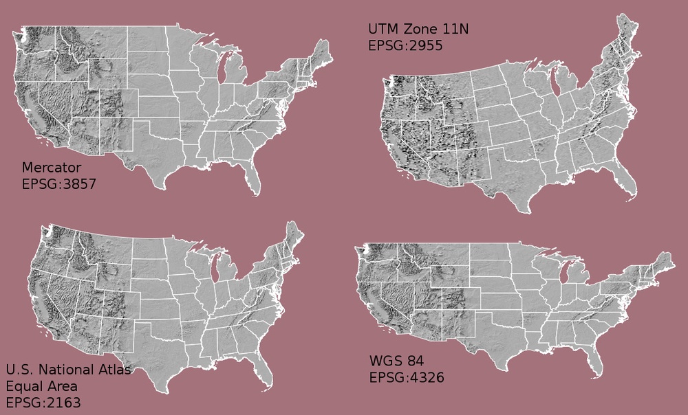
now we define a CRS object
# Define the coordinate system that will be used. Here we show several examples:
myCRS1 <- CRS("+init=epsg:4326") # WGS 84
myCRS2 <- CRS("+init=epsg:4269") # NAD 83
myCRS3 <- CRS("+init=epsg:3857") # Mercator
myCRS3 <- CRS("+init=epsg:3413") # WGS 84 / NSIDC Sea Ice Polar Stereographic North
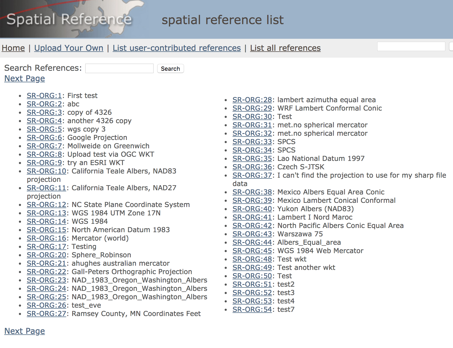
You can full reference list from spatialreference.org website.
assign the Coordinate Reference System (CRS) to our occ spatial object
crs(occ_final) <- myCRS1
crs(occ_final)
CRS arguments:
 +init=epsg:4326 +proj=longlat +datum=WGS84 +no_defs +ellps=WGS84
+towgs84=0,0,0
after defineing the CRS, we can do CRS projecitons
occ_final_projected <- spTransform(occ_final, myCRS3)
plot(occ_final)

plot(occ_final_projected)

after we transform a dataframe into a spatial object, we can still subset it by column; for example, here we only keep occurrences north of the Equator
occ_north <- subset(occ_final, occ_final@coords[,2] >=0)
plot(occ_north)

or we can subset by year
occ_1990 <- subset(occ_final, year ==1990)
plot(occ_1990)

2.6 Read/Write shapefile files
dir.create("temp")
shapefile(occ_final,"temp/occ_final.shp",overwrite=TRUE)
loaded_shapefile <- shapefile("temp/occ_final.shp")
Challenge: Download occurrences from GBIF and filter data
–select your favorite species
–only keepspecimenrecords
–only keep records that are collected between2000 & 2018
–only keep records that havevalid longitude & latitude
–make the occ spatial –assign WGS84 as the crs of the occurrences –save the spatial object as “myocc_final.shp” in folder “temp”Solution
library(dismo)
library(raster)

# download
myocc <- gbif(genus="Dasypus",species="novemcinctus",download=TRUE)

# filter
myocc_final <- subset(myocc,basisOfRecord=="PRESERVED_SPECIMEN" &
                            year >= 2000 & year <= 2018 &
                            !is.na(lat) & !is.na(lon)    )

# show number of records that are removed
nrow(myocc) - nrow(myocc_final)

# make it spatial
coordinates(myocc_final) <- ~ lon + lat

# define CRS
myCRS1 <- CRS("+init=epsg:4326") # WGS 84

# assign CRS to your occ
crs(myocc_final) <- myCRS1

# write shapefile
dir.create("temp")
shapefile(myocc_final,"temp/myocc_final.shp")