Raster data

Overview

Teaching: 10 min
Exercises: 10 min

Objectives

read/write raster data

raster metadata

raster resample

raster reclassification

raster calculation

raster correlation

3.1 Load libraries and set up folders

library("raster")
require(utils)
if(!file.exists("data")) dir.create("data")
if(!file.exists("data/bioclim")) dir.create("data/bioclim")
if(!file.exists("data/studyarea")) dir.create("data/studyarea")
if(!file.exists("output")) dir.create("output")

3.2 Download data

In our example, we use bioclimatic variables (downloaded from worldclim.org) as input environmental layers.

We use download.file() to directly download worldclim data, and used unzip() to unzip the zipped file

# download climate data from worldclim.org
if( !file.exists( paste0("data/bioclim/bio_10m_bil.zip")   )){
  utils::download.file(url="http://biogeo.ucdavis.edu/data/climate/worldclim/1_4/grid/cur/bio_10m_bil.zip",
                       destfile="data/bioclim/bio_10m_bil.zip"   ) 
  utils::unzip("data/bioclim/bio_10m_bil.zip",exdir="data/bioclim") 
}

3.3 Read/Write raster files

read one raster file at one time

test1 <- raster("data/bioclim/bio1.bil")
dir.create("temp")
writeRaster(test1,"temp/bio1.bil",overwrite=TRUE)
writeRaster(test1,"temp/bio1.tiff",overwrite=TRUE)

read 19 layers at one time

# search files with .bil file extension
clim_list <- list.files("data/bioclim/",pattern=".bil$",full.names = T)

# stacking the bioclim variables to process them at one go 
clim <- raster::stack(clim_list) 

You can write many different type of rasters:
.

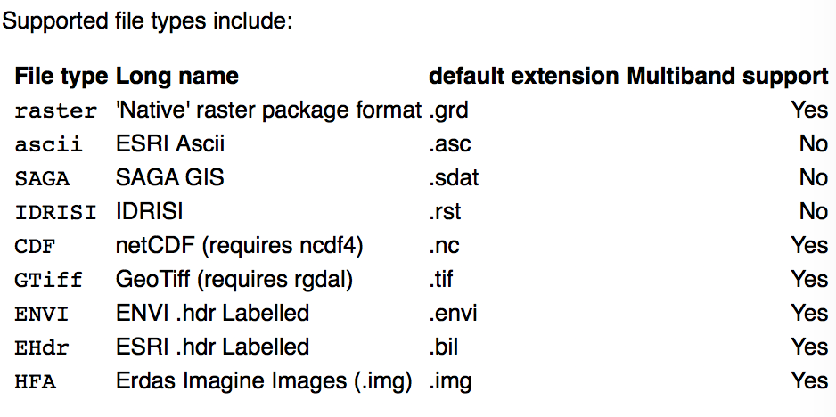3.4 Basic information of a raster

bio1 <- raster("data/bioclim/bio1.bil")
bio1

class       : RasterLayer 
dimensions  : 900, 2160, 1944000  (nrow, ncol, ncell)
resolution  : 0.1666667, 0.1666667  (x, y)
extent      : -180, 180, -60, 90  (xmin, xmax, ymin, ymax)
coord. ref. : +proj=longlat +datum=WGS84 +no_defs +ellps=WGS84 +towgs84=0,0,0 
data source : /Users/lablap/lesson_mac/_episodes_rmd/data/bioclim/bio1.bil 
names       : bio1 
values      : -269, 314  (min, max)

read number of rows

nrow(bio1)

[1] 900

read number of columns

ncol(bio1)

[1] 2160

read extent

extent(bio1)

class       : Extent 
xmin        : -180 
xmax        : 180 
ymin        : -60 
ymax        : 90 

read CRS (coordinate reference system)

crs(bio1)

CRS arguments:
 +proj=longlat +datum=WGS84 +no_defs +ellps=WGS84 +towgs84=0,0,0 

read resolution

res(bio1)

[1] 0.1666667 0.1666667

3.5 Resample raster

We want the new layer to be 10 times coarser at each axis (i.e., 100 times coarser). In essence, we are resampling the resolution from 10 min to 100 min.

bio1 <- raster("data/bioclim/bio1.bil")

# define new resolution
newRaster <- raster( nrow= nrow(bio1)/10 , ncol= ncol(bio1)/10 )

# define the extent of the new coarser resolution raster
extent(newRaster) <- extent(bio1)

# fill the new layer with new values
newRaster <- resample(x=bio1,y=newRaster,method='bilinear')

# when viewing the new layer, we see that it appears coarser
plot(bio1)

plot of chunk raster_manipulation

plot(newRaster) 

plot of chunk raster_manipulation

3.6 Reclassify raster layer

Reclassify as a binary layer: areas that are higher than 100 va. areas that are lower than 100

myLayer<- raster("data/bioclim/bio1.bil")

binaryMap <-   myLayer>= 100

plot(binaryMap)

plot of chunk reclassify_raster1

Use multiple threholds to reclassify

# values smaller than 0 becomes 0; 
# values between 0 and 100 becomes 1; 
# values between 100 and 200 becomes 2;
# values larger than 200 becomes 3;

myMethod <- c(-Inf,  0, 0, # from, to, new value
              0,   100, 1,
              100, 200, 2,
              200, Inf, 3)
myLayer_classified <- reclassify(myLayer,rcl= myMethod)
plot(myLayer_classified)

plot of chunk reclassify_raster2

3.7 Raster calculation

wet <- raster("data/bioclim/bio13.bil") # precipitation of wettest month
dry <- raster("data/bioclim/bio14.bil") # precipitation of driest month

# To calculate difference between these two rasters
diff <- wet - dry
names(diff) <- "diff"

# To calculate the mean between the dry and wet rasters
twoLayers <- stack(wet,dry)
meanPPT1 <- calc(twoLayers,fun=mean)
names(meanPPT1) <- "mean"

# the following code gives the same results
meanPPT2 <-  (wet + dry)/2
names(meanPPT2) <- "mean"

layers_to_plot <- stack(wet, dry, diff, meanPPT1,meanPPT2)
plot(layers_to_plot)

plot of chunk raster_calculation

3.8 Correlations between layers

# search files with *.bil* file extension
clim_list <- list.files("data/bioclim/",pattern=".bil$",full.names = T)

# stacking the bioclim variables to process them at one go 
clim <- raster::stack(clim_list) 

# select the first 5 layers
clim_subset <- clim[[1:5]]

# to run correlations between different layers
raster::pairs(clim_subset,maxpixels=1000) # the default is maxpixels=100000

plot of chunk raster_correlation

Challenge: download and process worldclim data

–download worldclim_V1.4 10m resolution bioclimatic layers
–read BIO5 (Max Temperature of Warmest Month) & BIO6 (Min Temperature of Coldest Month)
–calculate the difference between the two layers
–save the difference as difference.tiff in folder temp
Solution
dir.create("data")
dir.create("data/bioclim")

# download 
utils::download.file(url="http://biogeo.ucdavis.edu/data/climate/worldclim/1_4/grid/cur/bio_10m_bil.zip",
                      destfile="data/bioclim/bio_10m_bil.zip"   ) 
utils::unzip("data/bioclim/bio_10m_bil.zip",exdir="data/bioclim") 

# load rasters 
library(raster)
bio5 <- raster("data/bioclim/bio5.bil")
bio6 <- raster("data/bioclim/bio6.bil")

# calculate the differences
difference <- bio5 - bio6

# save the raster file
dir.create("temp")
writeRaster(difference,"temp/difference.tiff")

previous episode

next episode